The old formula that everyone uses for customer lifetime value (LTV)) –average gross profit per customer divided by churn – ceases to work properly when you have very long customer lifetimes and negative churn. LTV can become infinite, which clearly doesn’t reflect reality. This post offers a new way to calculate LTV based on discounted cash flow analysis that takes into account the risks associated with revenue that is far off in the future, and the time value of money. The resulting LTV can help companies better understand and manage their future revenue streams and it much more accurately reflects what an investor would pay for that future flow of cash.
Most of the content in this article is aimed at SaaS companies that are past the point where they have a repeatable, scalable and profitable sales process, and are well into their expansion phase. If you’re an early stage SaaS startup, still trying to get product/market fit, or experimenting with different ways to make your marketing and sales predictably repeatable and scalable, it is useful to play around with CAC and LTV to get a feel for where you are. But it’s important to note that these formulae will only yield meaningful results when your sales and marketing process and costs are predictable and scalable. Instead of spending too much time obsessing over CAC and LTV, rather focus your energies on solving the problems of improving product/market fit, and making your customer acquisition repeatable, scalable and profitable.
My apologies that there are some complex looking formulae in this article. We have provided a summary below of the key concepts, and a link* to jump straight to the spreadsheet to model your own LTV. For those interested in understanding the theory behind this model, we provide our usual detailed explanation below.
Summary
For subscription-based businesses who have “negative churn” (they expand revenue from retained customers at a greater rate than lost revenue from churn), you need new formulae to calculate LTV that includes both this expansion rate and churn.
In addition, because you are modeling revenues that will occur far in the future, you will need to apply a discount rate to account for the risks and time value of money. We recommend using a 10% discount rate, but this may differ depending on your own cost of capital.
This approach provides a lower, but more accurate view of your LTV. We have previously recommended your LTV to CAC ratio be greater than 3. However, we will be working with SaaS companies to understand the impact of this lower LTV calculation and will provide an updated recommendation in a future post.
Payback period does not change, and we still recommend a 12 month payback period unless you have easy access to a lot of capital. In that case, your payback period may be 18 months or longer.
Data you’ll need to model this new LTV, using the spreadsheet tool below:
- Average starting contract revenue per account
- Gross margin (this should include customer support and account management time to retain and upsell)
- Churn rate
- Growth rate for retained customers
**These #s can be monthly or annual #s, rates.
Real World Model
A more detailed second model in the spreadsheet linked below allows you to input data to reflect how churn and growth rates change over the life of a cohort of customers. You can input this data for whatever time period you have (first year, 18 months, 2 years, etc.) But, don’t obsess over the accuracy of this data and just use the best data you have. The model is much less sensitive to inputs in the far future; it’s more important to ensure your first year or two of assumptions are accurate.
Free Spreadsheet Attached
For those readers interested in modeling their own LTV, an Excel spreadsheet is attached. Click this link to download*.
*Spreadsheet updated 2/23/16 – errors corrected in Cell B78 on Real World Model tab.
Introduction
All of my regular SaaS/subscription economy readers know that one of the core concepts that I stress is the idea of measuring Unit Economics at the customer level to help entrepreneurs figure out if they have a good business, and if not, what they need to focus on to improve it. Unit economics is a simple concept where we look to make sure that the profit we are getting from a customer over their lifetime (LTV) is greater than the cost to acquire a customer (CAC). This is needed because in the early days of a fast growing SaaS/subscription business, the EBITDA losses can be huge, and investors and board members need a new kind of tool, that is not provided in the traditional accounting reports, to help them recognize the difference between the good businesses that will eventually produce great profits, and the bad businesses that will never turn a profit. (For more details on this topic, see SaaS Metrics 2.0.)
Those posts, and several others, focused on the importance of retaining customers, and trying to get to “negative churn”. It is this negative churn that now requires us to develop more complex measurements to understand future cash flows.
Traditional Churn and LTV
To study churn, we need to look at a particular group of customers that signed up in a particular time period. We refer to these groups as cohorts. So you might have a Jan 2014 cohort which is comprised of all the customers that signed up in Jan 2014. We will then want to track how many customers we retain, and how the revenue for each cohort evolves over time. Here is a graph that shows what happens to the number of customers in a particular cohort over several years with three different monthly Customer Churn Rates.
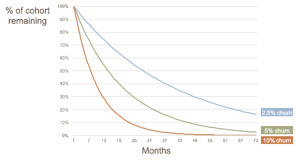
As you may be able to tell, the graph is an exponential decay, and for exponential situations, we can use a simple formula to get at the average Customer Lifetime:

And from there, we can simply multiply that average lifetime by the average amount of Gross Profit that we make from each customer every year to get to LTV:

Filling this out with the math for average customer lifetime, and gross profit per account, we get this formula:
 (ARPA is the Average Revenue per Account)
So far, we have only looked at a simple version of churn, which is the rate at which our customers churn. However, things are more complicated when we look at how revenue behaves when you have churn.
Why Dollar Retention Rate (DRR) is different to Customer Retention Rate (CRR)
Imagine a situation where we start the year with two customers, one small and one large:

Now let’s look at what happens if we lose Customer 1:
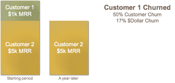
Our Customer Churn was 50%, but our Dollar Churn was only 17%. So we see that these two numbers behave differently, and need to be tracked separately to understand the full picture of what is going on in the business. This points out an obvious fact: it is more important to retain your larger customers than it is to retain your smaller customers.
Now let’s look at what happens if we were able to expand the revenue we are getting from Customer 2 from $5k to $7k:
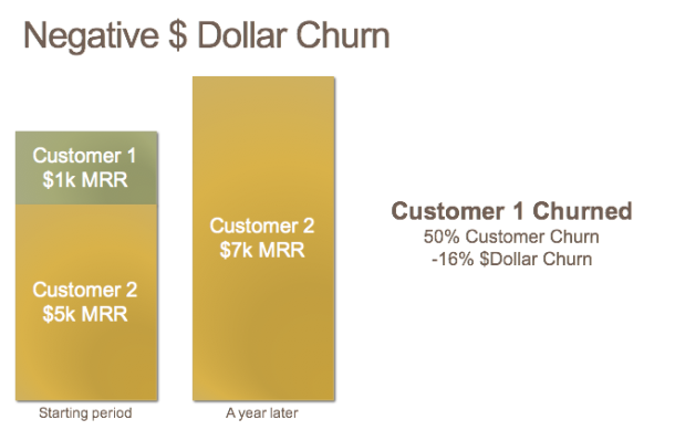
Something very interesting has happened here: the expansion revenue of $2k from remaining customers was greater than the $1k that we lost from the churned customers, and we have Negative Dollar Churn, even though the Customer Churn remained at 50%.
This is an extremely powerful concept, which I have written about before here: Why Churn is SO critical to success in SaaS. It does raise an interesting question, which is how do we get our current customers to expand, and that requires that we have either variable pricing, and/or additional product modules to sell. I have covered this topic in a prior post on Multi-Axis pricing.
CRR and DRR
So far we have talked about Customer Churn and Dollar Churn. There are two other terms which you might see used, which are the counterparts to churn:
- CRR (Customer Retention Rate) which is equal to 1 – Customer Churn Rate
- DRR (Dollar Retention Rate) which is equal to 1 – Dollar Churn Rate
So a business that has a negative churn rate, will have a Dollar Retention Rate of greater than 100%. These are some of the very best SaaS business out there. Examples of DRR greater than 100% include: Zendesk: 123%, NewRelic 115%, Box: 130%, Rally Software 127%. (For more public company retention rates you might like to check out this article by Pacific Crest.)
Negative Churn invalidates the LTV formula
In the LTV formula above, I kept things simple by using the term “Churn Rate”. But I should have been more precise and used the term Dollar Churn Rate to avoid confusion with Customer Churn Rate. But now we have a problem, if we insert a negative value in the LTV formula, we don’t get the right answer. And you can tell quite easily without a formula, that if our cohort kept growing at 16% every year (which is what is implied by a negative 16% churn rate), then we would have an infinite future revenue stream that would grow and grow from this cohort.
Our first attempt to model this phenomenon, showed that there is a point where the customer churn starts to bring down the revenue. Here’s a graph showing what would happen if you had a cohort of 100 customers that initially started paying you $100 a month, but each remaining customer increased their payment by $5 every month. The monthly Customer Churn Rate is 3%:
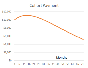
In case of interest, the formula used to compute this graph is:
a = initial ARPA per month x GM %
m = a fixed $ amount of monthly growth in ARPA per account (not compounding)
c = Customer Churn Rate % (in months)
The formula would work equally well for yearly values.
(Note: there is a huge simplification in this formula that we will address later: it assumes a fixed linear expansion in revenue over time, and in most cases this won’t be how expansion revenue happens.)
Using DCF to account for Risk and Time Value of Money
Given that so much of the customer value in this situation occurs way in the future, where there are risks of the market changing, new competition, technology platform changes, etc. it makes sense that we should factor in that risk in some way when computing LTV. Similarly, we all know that if we were offered a dollar in ten years time, we’d value it far lower than a dollar today. Applying a discount to future cash flows is the accepted way to model this phenomenon.
Here is what happens if we apply a 10% annual discount to the cash flows of a SaaS business with 10% annual dollar churn:
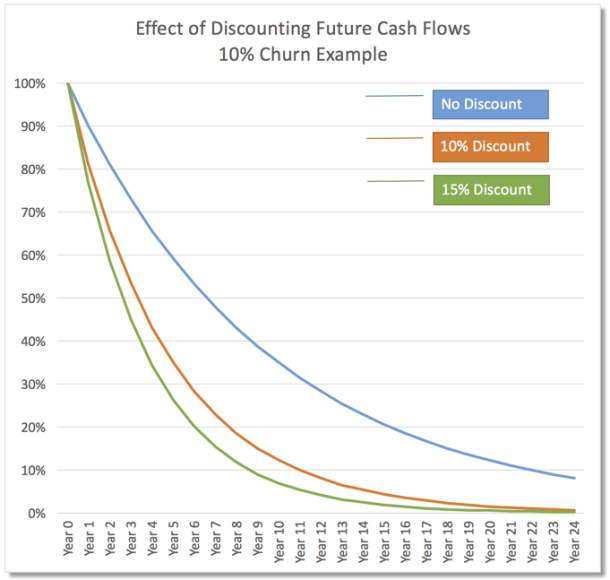
The vertical Axis represents the percentage of the initial cohort contract value, and how it drops over time with a 10% annual churn rate. Then the orange and green lines show the impact of adding discounting of future cash flows to the blue baseline.
This shows what we were expecting to achieve: a lower value associated with cash flows that are farther away in time, reflecting future risks and the time value of money.
This far more accurately reflects what an investor would be willing to pay today, for that flow of cash going into the future.
True LTV: DCF applied to a Negative Churn Scenario
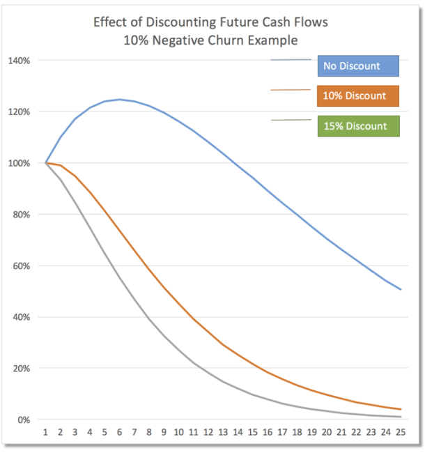
The graph below shows what happens to Cash Flows in a Negative Churn scenario:
- Churn rate of negative 10%, as a result of the following two variables:
- Customer Churn is 10% annually
- Remaining customers increase their spend by 22% of the original contract amount every year (note this is linear, not compounding and exponential)
This requires us to come up with a new formula for LTV:
Where G is the growth rate for the customers that have not churned, and K is defined by the following formula:
Where Churn is the Customer Churn rate.
Note: the formula above is included in the provided spreadsheet, on the Tab called LTV Calculator.
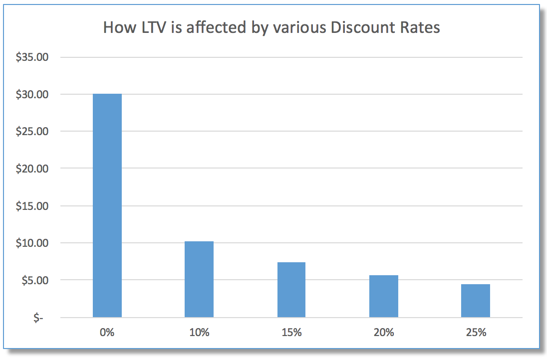
Using this formula, we can see that the LTV, for a starting contract with $1 of gross margin, changes as follows:

The left hand bar shows LTV when there is no discount applied. All the CFOs that I talk to know that this number is too high. Then the four bars to the right show what happens to LTV when we apply discounts to future cash flows.
What is the right Discount Rate?
All financial theory is consistent about one thing: every time managers spend money they use capital, so they should be thinking about what that capital costs the company. There can be many sources of capital, and the weighted average of those sources is called WACC (Weighted Average Cost of Capital). For most companies it’s just a weighted average of debt and equity, but some could have weird preferred structures etc. so it could be more than just two components.
The discount rate that is used in a DCF should be your company’s Weighted Average Cost of Capital (WACC).
If we were looking at the true cost of capital, we’d suggest the following discount rates to use:
- 10% for public companies
- 15% for private companies that are scaling predictably (say above $10m in ARR, and growing greater than 40% year on year)
- 20-25% for private companies that have not yet reached scale and predictable growth
The earlier the stage of the startup and the greater the risk in the business, the higher the discount.
However, there is an argument to be made that startup SaaS companies shouldn’t be using a different discount rate to public SaaS companies, as their goal is to show that they have the needed unit economics to eventually become a public company. And investors, board members and management will want to compare their LTV numbers to other larger companies. So given that thinking, we’d be inclined to suggest that the whole industry standardize on using one way of calculating LTV using discounted cash flow, and use one discount rate, which would probably be 10%. That way you could compare private company LTV numbers with public company LTV numbers. We are charting new territory with this analysis, so it will be interesting to hear readers’ feedback on this question.
We have provided the detailed thinking, formulae and calculations behind those numbers on the following page: “How to calculate the discount rate for use in a DCF” Here we go into how to calculate WACC. A key component of WACC is the cost of equity, which is computed using CAPM, the Capital Asset Pricing Model to arrive at a discount rate. This is explained in more detail in that article for those who have the curiosity to dig deeper.
Impact of DCF on the LTV:CAC Ratio
My regular readers will know that I have long recommended that SaaS startups should have an LTV : CAC ratio of greater than 3. Given that we will now be looking at lower LTV numbers because of using DCF, this recommendation will need to be changed to a lower number. I don’t yet have a firm point of view on what this new ratio should be, and will be spending time with a bunch of companies that decide to use the DCF version of the LTV formula to watch what this does to their LTV:CAC ratio before making a final recommendation.
However, my other recommendation, that SaaS companies should measure their Months to recover CAC remains a great metric to understand whether your company has good unit economics. For companies looking to optimize their cash flow, I have recommended that they try to recover CAC in 12 months or less. But if your startup is able to cheaply raise a lot of capital, you may be able to relax this, and recover CAC in 18 months, or even a bit longer.
Introducing CORE – Cost of Retention and Expansion
Most readers will realize that it requires Account Managers time and effort to retain customers, and additional sales effort to get expansion revenue. In most organizations this cost is part of the Sales expense, which may be fine for accounting purposes, but is not going to reflect correctly in our CAC and LTV calculations, as it will show up as a misleading number in CAC. To give you a sense for this, imagine a mature SaaS company with a large installed base producing about $100 million in recurring revenue. To keep that installed base happy, and to maximize retention, that company will likely have a large number of Account Managers. If the cost of these Account Managers shows up in CAC for newly added customers, it will make the CAC number much higher than it really is.
The solution is to move the costs of these Account Managers, plus any extra sales people that are needed to generate expansion revenue in that customer base, into the LTV side of the equation, as these are really a true Cost of Retention and Expansion (CORE) and should be treated similarly to COGS when computing the Gross Margin for that recurring revenue. So in the formulae above*, when computing Gross Margin %, don’t forget to include both COGS and CORE.
How to calculate CORE and Gross Margin % for an average customer
You will likely know how many customers a single Account Manager can handle. And if you have specialist Expansion Sales Reps, again, you will likely know how many customers they can handle. As an example, let’s say that our organization has both Account Managers and Expansion Sales Reps. In that situation CORE for a single customer is calculated as follows:
And Gross Margin % now becomes:

Where COS is the Cost to Serve a single customer (hosting costs + support costs).
Understanding the effectiveness of an Expansion Revenue Salesforce
If you have dedicated sales people that only work on generating expansion revenue, and they are in addition to the Account Managers, it will be interesting to see what the CAC and LTV is for expansion revenue. My recommendation would be to create a second parallel tracking system to track these two elements. That will allow you to figure out the return on this investment, and compare it to other potential investments that you could make elsewhere in the business.
The Real World is more Complicated!
All of the above formulae make some key assumptions that typically don’t hold true in the real world:
Assumption 1: Your customers will churn in an exponential decay month after month.
In the real world, churn curves have quite different shapes from one company to another, and frequently improve over time. For instance, many companies using annual contracts will have little churn until the end of the contract periods.
Assumption 2: Your remaining customers will expand their revenue in a linear fashion
In the real world, this is highly unlikely to be the case, and will also vary a lot from company to company. It’s possible that you might see a linear increase if they have some kind of pricing axis such as user seats that increases predictably over time. Other factors such as upsell of new modules will be very non-linear, and will occur at odd times. Some companies might see a lot of expansion in the early days, and then it could taper off.
Assumption 3: Your Gross Margin % will remain constant over time
In the real world, most SaaS companies are able to improve their gross margins substantially in the years before they hit true scale (around $150m in ARR). If it is clear that your gross margins will be increasing predictably, you may find it valuable to model this as a changing variable.
Revenue versus Billings
Another important factor to note is that the formula above focuses on the timing of revenue, which could be very different to how cash is collected. Many startups are able to bill a year in advance, which means that the cash flows would actually be quite different to the revenue flows. Applying DCF to the revenue instead of the actual cash flows would penalize those companies somewhat. Trying to build a formula to take this into consideration would add too much complexity, and we don’t think that the difference warrants that extra complexity. But if you were looking to be entirely accurate about this, you could modify the provided spreadsheet to use cash flows (i.e. billings) instead of revenue.
Modeling the real world
The spreadsheet that accompanies this article provides a way to model your real world experiences on how two of these variables will change. Just go to the “Real World Model” tab of the spreadsheet*, and enter in your values for the churn and expansion as you observe (or believe) they change over time from your cohort analysis. It’s unlikely that you will know more than the one to three years of data, so enter only what you do know, and then use the Residual Value formula to predict the other years.
How should SaaS Startups react to this article
Don’t obsess over getting to the last level of accuracy here. We are using a formula to predict the future, and the future, by it’s very definition is not predictable. So recognize that the value in this analysis is to get enough accuracy to make useful business decisions, such as what factors to look at to improve profitability, which customer segments are most profitable, and which have problems that need addressing, etc.
Make sure you have the data you need to understand Churn, Expansion and LTV
There is one thing that all SaaS companies should do immediately after reading this article, if they haven’t done so already: build a database to track revenue by individual customer by month that can be used with an analytics tool to analyze cohorts. You will need to be able to look at all customers that started in a particular month (a cohort), and track customer count and revenue for that cohort over time. Also make sure to tag each customer with attributes such as “Enterprise”, “SMB” so that you can look at how churn and expansion varies over time for the different types of customers. This analysis will become extremely valuable at showing you which are your most profitable customer segments, and where you need to do work to fix issues.
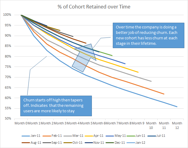
This data will allow you to get Cohort graphs such as the one shown below, that will allow you to understand the shape of how your customer count and revenue decay over time. To create this graph, we are simply overlaying multiple cohorts data on top of each other, and treating their starting month as Month 0. The shape of these curves can be used with the spreadsheet model provided to calculate your real Customer Lifetime Value (LTV).
Conclusion
I have had many questions over the years from SaaS entrepreneurs and CFOs about how to calculate LTV when they have negative churn. They clearly realized the that old formula of Average Gross Profit per Account divided by Churn did not work in their situation. This article and the attached spreadsheet hopefully addresses that question. My apologies that there are some complex looking formulae in the article. If you are a reader who doesn’t like the look of those, simply download the spreadsheet*, and enter your own data into LTV Calculator.
I am really interested in hearing readers’ feedback on the ideas expressed in this article. Please leave me comments below.
*Spreadsheet updated 2/23/16 – errors corrected in Cell B78 on Real World Model tab
My thanks to my partner Stan Reiss, who co-authored this piece with me, providing all the expert math help. Thanks also to Joe Ferrero, Sai Ho and Alan Black of Zendesk for contributing their insights.


